Goals
Marine pollution is a condition where marine waters are getting polluted from i ndustrial, agricultural, residential waste, and some invasive organisms. Based on the data I have collected, I decided to make a clustering model that will divide data into 2 cluster, polluted water and non-polluted water.
Data Dictionary
1. Trash Pollution :
The level of manufactured products such as plastic that end up in the ocean.
2. Oil Concentration :
The amount of oil residue in waters.
Oil cannot dissolve in water and forms a thick sludge in the water.
The amount of harm caused depends on how an organism is exposed and to how much oil.
3. Bacteria Level :
The level of bacteria in Colony Forming Units (CFU) per 100 mL of water.
Bacteria is a microorganism that live in diverse environment and can in soil, ocean, and human guts.
The presence of bacteria can be beneficial while some that is pathogenic can be harmful.
4. Algae Concentration :
The concentration of algae living in the waters.
Algae are a diverse group of aquatic organisms that can conduct photosynthesis.
Most algae are harmless and an important part of the natural ecosystem,
but under certain conditions, it can harm humans, fish, and other animals.
5. Humidity : The concentration of water vapor present.
6. Wind Direction : The surrounding wind direction in degree.
7. Air Temperature :
The surrounding air temperature in Celsius.
An increase in the air temperature will cause water temperatures to increase as well.
8. Polluted : Whether the water is polluted or not (Yes, No).
Dataset
You can download the dataset on Github .
Source Code
Library
1. SparkSession :
SparkSession is the entry point for interacting with Spark SQL and allows you to
create DataFrames, execute SQL queries, and access various Spark functionalities.
2. when : to define conditional expressions in PySpark DataFrame operations.
3. KMeans : KMeans is an algorithm used for unsupervised clustering,
where it groups similar data points into clusters based on their feature similarity.
4. StandardScaler and VectorAssembler:
These library are used for feature engineering tasks.
VectorAssembler combines multiple feature columns into a single vector column,
and StandardScaler scales the input features to have zero mean and unit variance.
5. matplotlib : popular data visualization library in Python.
It allows you to create various types of plots and charts.
Import Data and Preview
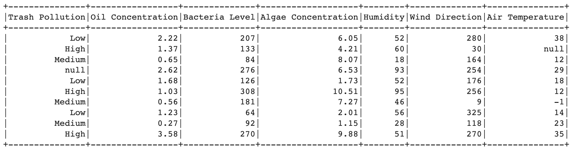
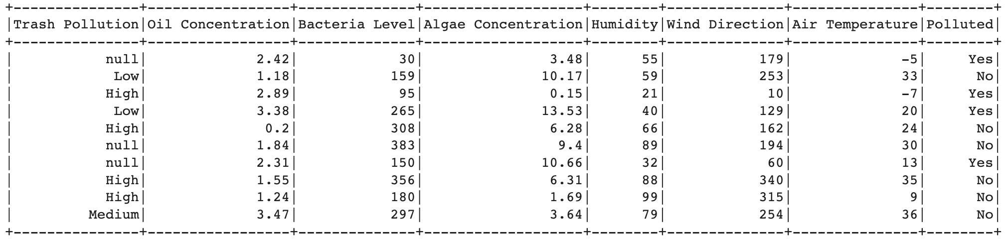
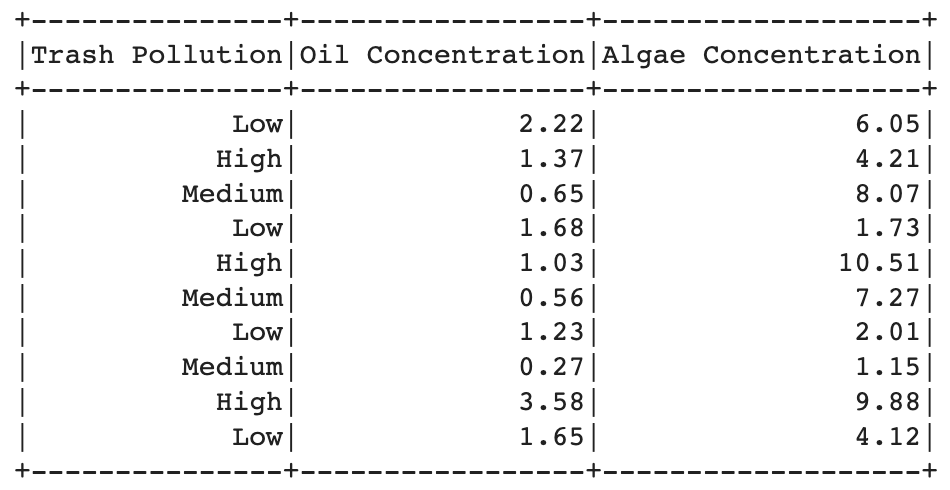
After import the library, then import the dataset. Here is the code for loads the training and testing data from CSV files using spark.read.csv(). The inferSchema=True option enables automatic inference of column types, and header=True indicates that the first row of the CSV file contains column headers.
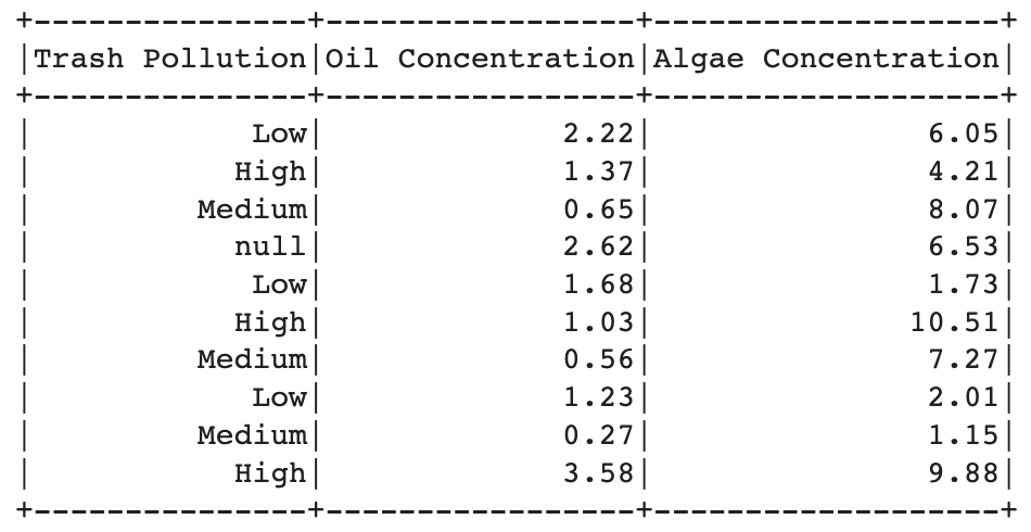
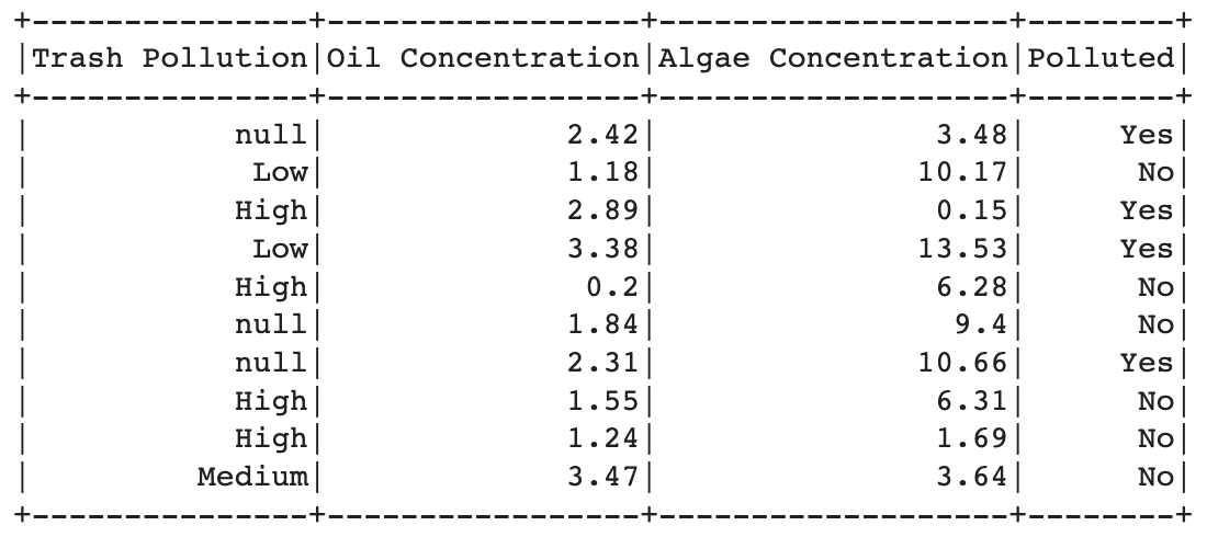
Select Features
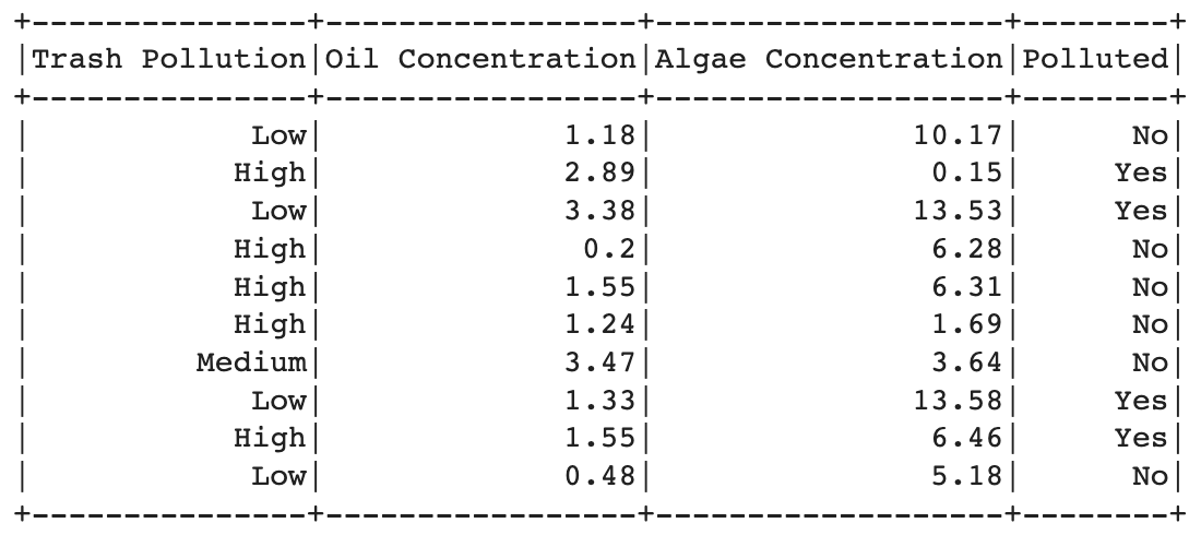
After that, selects specific columns from the loaded data, including "Trash Pollution", "Oil Concentration", "Algae Concentration", and "Polluted", for both the training and testing datasets.
Preprocessing
In this step, we used na.drop() to remove any rows with missing values from the training and testing datasets.
Transformation
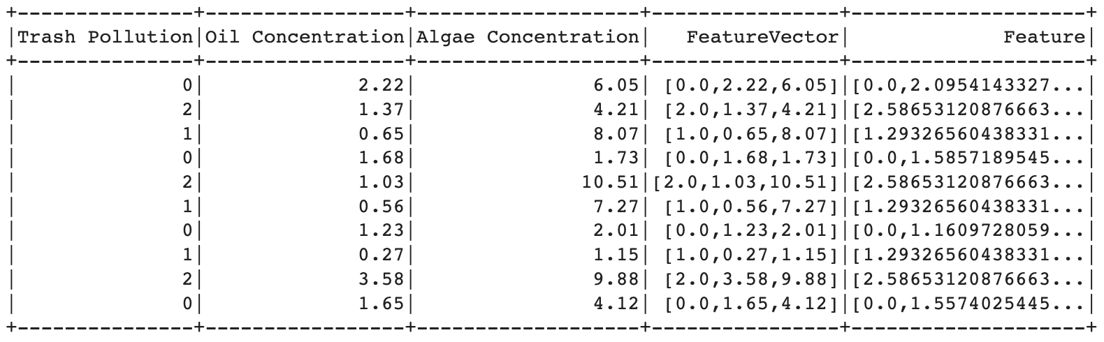
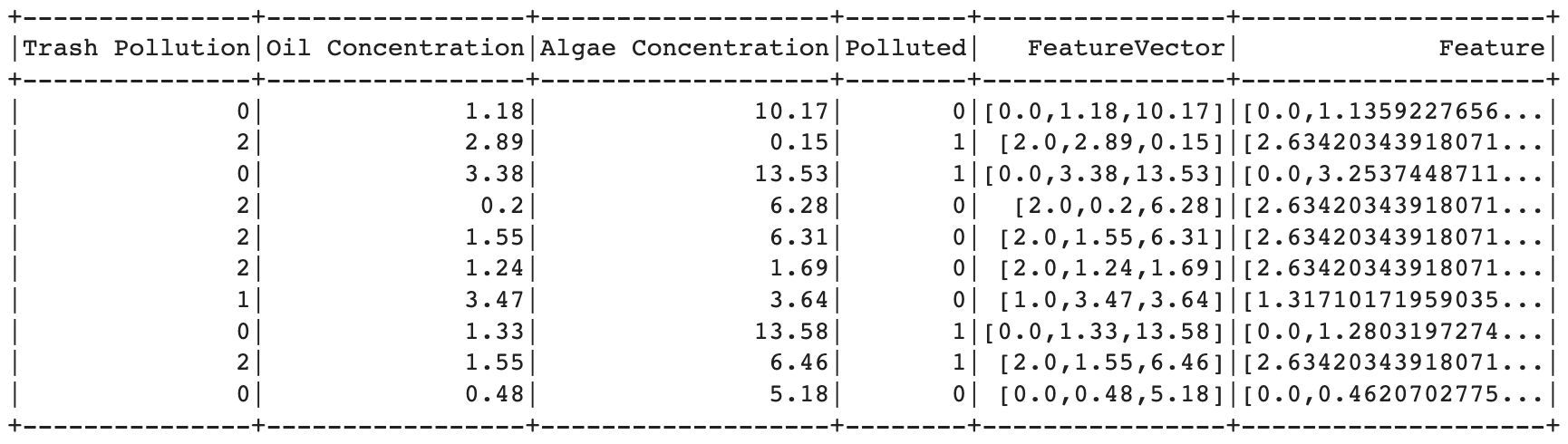
In this step, transforms the data by converting categorical values in the "Trash Pollution" column to numerical values using the withColumn() method and when function. The "Low" category is mapped to 0, "Medium" to 1, and any other category to 2.
Normalization
Then, we normalized the data using VectorAssembler to assemble the selected feature columns into a single vector column called "FeatureVector". And, StandardScaler is applied to scale the "FeatureVector" column, producing a new column called "Feature" with standardized values. This normalization step ensures that all features are on a similar scale, which can be important for certain machine learning algorithms.
Generate Model
A k-means clustering model is created using KMeans from pyspark.ml.clustering.
The number of clusters (k) is set to 2, and the "Feature" column is specified as the input feature column for clustering.
The model is trained using the training dataset with the fit() method.
The trained model is used to make predictions on the testing dataset using the transform() method,
resulting in a new DataFrame called "predict" that includes the original features
and a "prediction" column indicating the predicted cluster for each data point.
The "predict" DataFrame is converted to a Pandas DataFrame using the toPandas() method,
which brings the data to the driver node in a local Pandas DataFrame.
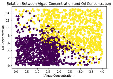
Visualization
In this step, visualize the data using matplotlib.pyplot. It creates a scatter plot using the "Oil Concentration" and "Algae Concentration" columns as the x and y axes, respectively, and colors each point based on the "prediction" column. The resulting plot shows the relation between algae concentration and oil concentration based on the clustering results.
Model Testing and Evaluation
Model testing and evaluation are done by comparing the "Polluted" column in the Pandas DataFrame with the "prediction" column.
The code counts the number of correct predictions and calculates the accuracy by dividing the number of correct predictions by the total number of predictions.
The calculated accuracy is printed as a percentage using f-string formatting.
Accuracy : 80.88004190675746% = 80.88%